PyStan 体验

安装环境

Python 3.6.4 |Anaconda, Inc.| (default, Dec 21 2017, 21:42:08) [GCC 7.2.0] on linux

直接运行

pip install pystan

Example: parallel experiments in eight schools

This example is from Section 5.5 of Gelman et al. (2013).

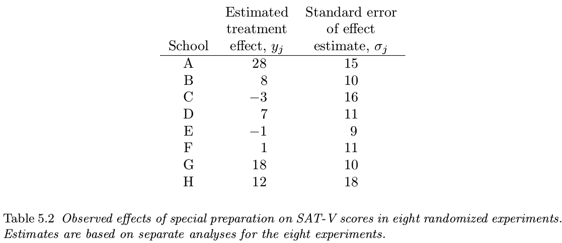
ETS perform a study to analyze the effects of special coaching programs on test scores. The results of the experiments are summarized in the following table:

A pooled estimate

This pooled estimate is 7.7, and the posterior variance is $(\sum_{j=1}^81/\sigma_j^2)^{-1}=16.6$. Thus, we would estimate the common effect to be 7.7 points with standard error equal to $\sqrt{16.6}=4.1$, which would lead to the $95\%$ posterior interval $[-0.5, 15.9]$.

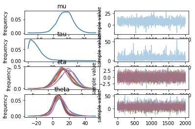
Posterior simulation under the hierarchical model

Compute the posterior distribution of $\theta_1,\ldots,\theta_8$.

The Bayesian analysis of this example not only allows straightforward inferences about many parameters that may be of interest, but the hierarchical model is flexible enough to adapt to the data, thereby providing posterior inferences that account for the partial pooling as well as the uncertainty in the hyperparameters.

import pystan

schools_code = """
data {
    int<lower=0> J; // number of schools
    vector[J] y; // estimated treatment effects
    vector<lower=0>[J] sigma; // s.e. of effect estimates
}
parameters {
    real mu;
    real<lower=0> tau;
    vector[J] eta;
}
transformed parameters {
    vector[J] theta;
    theta = mu + tau * eta;
}
model {
    eta ~ normal(0, 1);
    y ~ normal(theta, sigma);
}
"""

schools_dat = {'J': 8,
               'y': [28,  8, -3,  7, -1,  1, 18, 12],
               'sigma': [15, 10, 16, 11,  9, 11, 10, 18]}

sm = pystan.StanModel(model_code=schools_code)
fit = sm.sampling(data=schools_dat, iter = 1000, chains = 4)

# return a dict of arrays
la = fit.extract(permuted=True)
mu = la['mu']

# return an array of three dimensions: iterations, chains, parameters
a = fit.extract(permuted=False)

# plot
fit.plot()